Chapter 1: Introduction to Machine Learning and ERM

In the previous article, I discussed the concept of PAC Learning. Today, I will introduce the framework of a Machine Learning problem, focusing on Empirical Risk Minimization (ERM).

Every machine learning task revolves around analyzing data. Our goal is to input data into the system to uncover patterns. It's essential to remember two key points:

1. If you had complete knowledge of the data distribution, machine learning would be unnecessary.
2. Machine Learning isn't merely about predicting the class of a sample; it’s about developing a prediction rule that aids in making that classification.

Even a basic if-else program can classify data based on established rules. The essence of machine learning lies in discovering a hypothesis that can be consistently applied to an unknown data distribution, thereby improving prediction accuracy.

Imagine you find yourself on an island abundant with papayas. Your objective is to form a hypothesis to determine whether a papaya is delicious by just inspecting or handling it. Developing this intuition requires experience; tasting numerous papayas will help you make better predictions about their flavor.

The tastiness of a papaya might be influenced by various factors such as color, size, shape, texture, hardness, the region of growth on the island, the tree's size, the amount of sunlight, and the water supply received. Numerous possibilities contribute to a papaya's ultimate flavor.

Based on this scenario, the fundamental components necessary for machine learning are:

• Inputs:

  • A domain set X that represents the vector space of inputs. In our case, this could include information about the color, shape, size, and hardness of the papaya, along with its growth location and other relevant features.
  • A Label Set Y, which indicates whether the papaya is tasty (1) or not (0).
  • A Training Set, as you need to taste many papayas to form your hypothesis about their tastiness. This collection of papayas is termed Training Data in machine learning.

• Output:

  The output from the machine learning model is a hypothesis or prediction rule, denoted as ( h: X rightarrow Y ), indicating that the hypothesis takes an input from the domain X and predicts an output from domain Y, which consists of values 0 or 1.

For those new to machine learning, it may seem confusing how Y can serve as both an input and the result predicted by the hypothesis. This is a characteristic of a specific type of machine learning known as Supervised Learning. The algorithm learns from training data that includes samples from domain X paired with the correct labels from domain Y. Once the hypothesis is established, it can predict the label for previously unseen data from domain X, allowing you to determine if a new papaya is tasty without tasting it.

As you navigate the island, you cannot predict what kind of papaya you will encounter next. It simply hangs on a tree, waiting for you to collect it. This uncertainty mirrors the unknown distribution from which your papayas come, referred to as the data generation model. When nature produces a papaya, it generates data for you to analyze.

Let’s denote this unknown distribution as ( P_x ). Assume there exists a function ( Y = f(x) ) that provides the definitive answer regarding whether a papaya is tasty. Understanding this assumption will be crucial later.

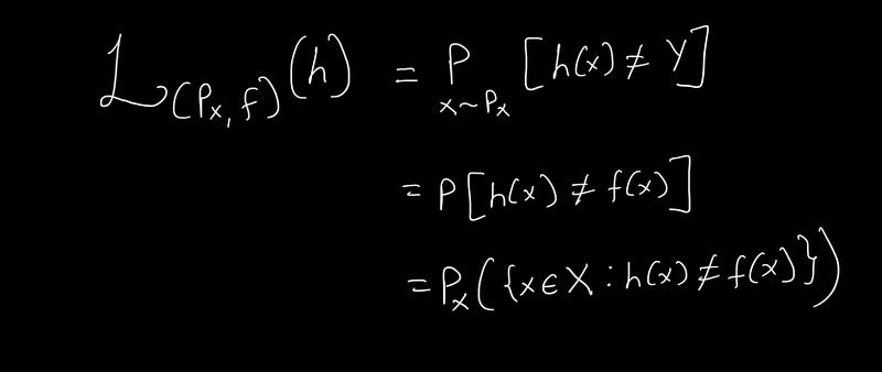
How can you assess the accuracy of your hypothesis? This is where the concepts of Loss or Risk come into play, defined as follows:

The loss ( L(P_x, f)(h) ) indicates the risk associated with the hypothesis. The notation ( (P_x, f) ) signifies that the loss is assessed concerning the true distribution ( P_x ) and the correct labeling function ( f ).

The first term asserts that the loss equals the probability ( P ) where the hypothesis ( h(x) ) does not equal ( Y ). The subsequent step emphasizes that ( Y = f(x) ). Notably, ( x sim P_x ) indicates that the sample ( x ) originates from the distribution ( P_x ). The final interpretation generalizes that the Loss represents the probability of the hypothesis differing from ( f(x) ) for ( x ) drawn from domain X according to the distribution ( P_x ). This is a generalized loss concerning the true distribution.

Since we cannot ascertain the true distribution, as previously mentioned, we would not need machine learning if we could, we must adapt our loss measurement to the data we possess. We can define a risk based on the training data, termed Empirical Risk. The term "Empirical" signifies that it can be verified through observation rather than pure theory, highlighting that when measuring loss against observed data, we assess the Empirical Risk, represented as follows:

Here, the subscript ( s ) indicates that the loss is defined concerning the training data, and ( n ) represents the number of training samples.

Our goal is to identify a hypothesis ( h ) that, when evaluated against this Empirical Loss, yields the lowest possible loss value. This objective can be expressed as follows:

And this encapsulates the concept of the Empirical Risk Minimizer! Stay tuned for the next post :)