What if I told you that a single equation links the Mandelbrot set, squirrel populations, dripping faucets, neuronal firing, and thermal convection? You might find that hard to believe, but mathematics often reveals surprising truths.

Let’s delve into this intriguing concept.

Imagine modeling a squirrel population. This year, we start with X squirrels. What could next year's population be? A straightforward approach is to multiply the current population by a growth factor r. Thus, the population next year would be rX.

If r equals 2, it suggests that the population doubles each year. However, this assumption leads to unbounded exponential growth, which is unrealistic. To account for environmental limitations, we incorporate the term (1-X) into our equation.

The modified equation becomes rX(1-X), where X represents a fraction of the maximum population capacity, ranging from 0 to 1. As X nears 1, (1-X) approaches 0.

Let’s denote next year’s squirrel population as X? and this year's as X???. This leads us to the equation:

X? = rX???(1-X???)

This is known as the logistic map equation, and if you plot X? against X???, the result is an inverted parabola.

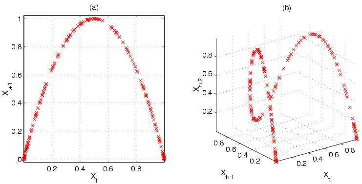
In this graph, t is used instead of n, but they represent the same concept.

This equation establishes a negative feedback loop: as the population surpasses X??? (this year), it decreases next year to X?.

Need more clarity? Let’s consider some examples.

Assume r is 3.4 and the initial population X??? is 0.3 (30% of the maximum). After calculation, we find the population rises to 0.816. However, if we take 0.816 as this year's population, next year it drops to 0.510, and subsequently rises to 0.849.

Interestingly, after several cycles, the population stabilizes between approximately 0.451 and 0.842, oscillating without significant change.

What about when r is around 2? The population stabilizes because two offspring replace their parents. For instance, if X??? is 0.35 and r is 2.34, next year's population becomes 0.532. Following iterations lead to a stabilization around 0.57, representing equilibrium.

Even if we alter the initial population, it will eventually converge to this equilibrium, which solely depends on r. A lower r means a lower equilibrium population; if r is below 1, the population trends to extinction.

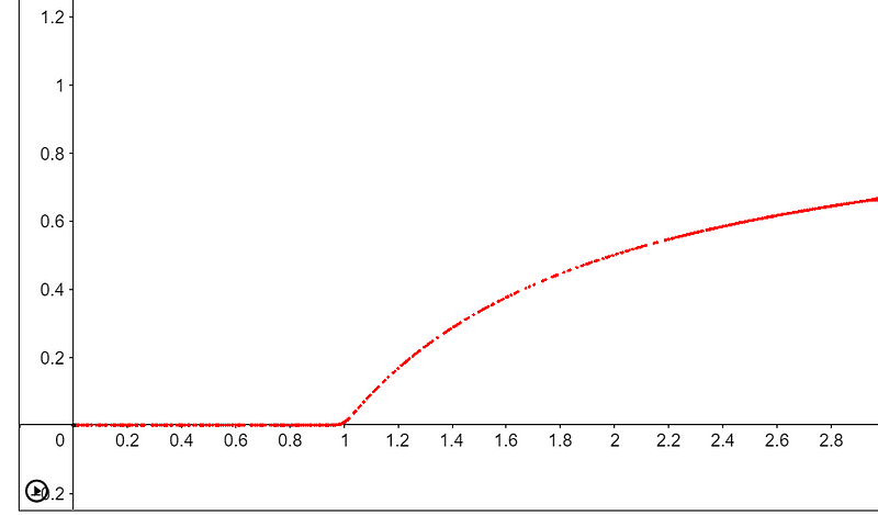
Now, let’s graph r (growth rate) on the x-axis against the equilibrium population on the y-axis. Initially, when r is less than 1, the equilibrium population is zero. But as r exceeds 1, the equilibrium population begins to rise.

Remarkably, when r surpasses 3, we observe oscillations. For r = 3.4, the equilibrium population fluctuates between 0.84 and 0.51 without settling, alternating each year.

As time progresses, this equilibrium divides into four distinct values, establishing a cycle every four years.

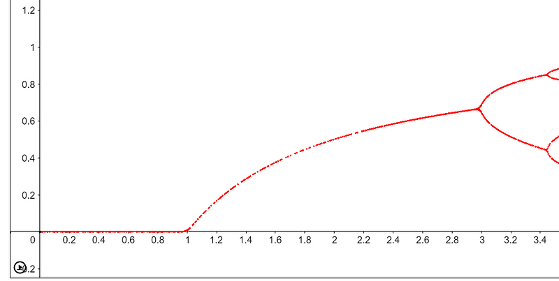
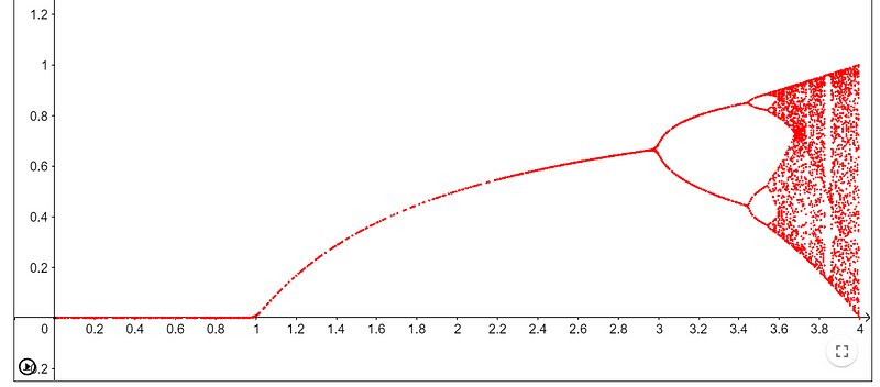
As cycles double, this phenomenon is termed period-doubling bifurcations. Increasing r results in cycles of 8, 16, 32, and beyond. When r reaches approximately 3.57, chaos reigns, leading to unpredictable population behaviors.

The population dynamics become erratic, so unpredictable that this principle has been utilized for generating random numbers in computing. Although non-repeating, if the initial values are known, predictions can still be made, classifying it as pseudo-randomness.

Notice the graph near r = 3.83 where order re-emerges, with the population repeating every three years. As r increases further, cycles expand to 6, 12, 24, leading back to chaos.

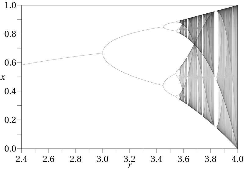
You might observe that this resembles a fractal, and you’re correct. Larger features repeat on a smaller scale.

The Mandelbrot set is perhaps the most well-known fractal.

Interestingly, the bifurcation diagram is a subset of the Mandelbrot set.

Isn't that fascinating?

So, what exactly is the Mandelbrot set?

It derives from the equation Z? = Z???² + C. Choose any number C in the complex plane and start calculating Z? from Z??? = 0. Iterate this process indefinitely.

If the results tend toward infinity, then that chosen C is not part of the Mandelbrot set. Conversely, if the values remain finite through endless iterations, it belongs to the set.

For instance, if C = 3, the iterations yield values that diverge to infinity, thus not part of the Mandelbrot set. However, if C = -1, the iterations oscillate between -1 and 0, confirming it as part of the set.

The Mandelbrot set visually represents the boundary between numbers that diverge and those that remain finite. To illustrate how these equations stabilize, we perform thousands of iterations and plot the iteration count on the z-axis, giving us the bifurcation diagram.

All numbers within the main cardioid converge to a single constant, while those in the main bulb oscillate between two values. Smaller bulbs oscillate between four values, and the chaotic regions appear at the edges of the Mandelbrot set. Notably, the medallion in the center of the needle region indicates where the bifurcation stabilizes briefly.

Isn’t this beautiful and perplexing?

Now, I assert that this equation governs species populations. This claim holds true, particularly under controlled conditions. Furthermore, this equation applies to a variety of scientific fields, often connecting seemingly unrelated areas.

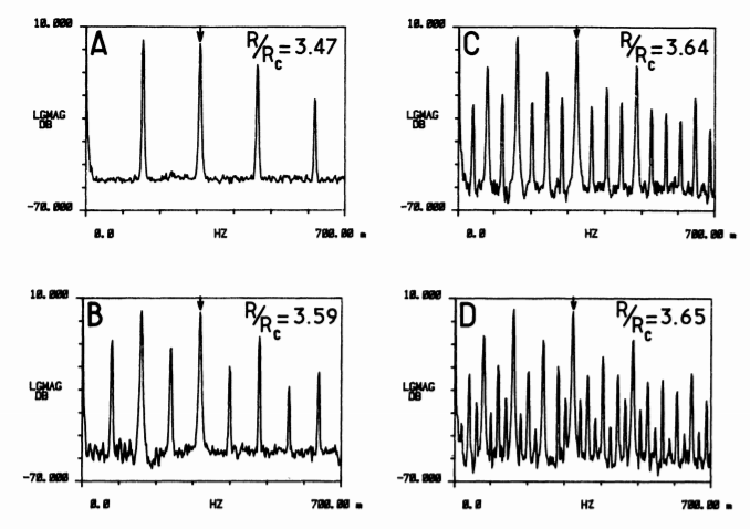
Albert J. Libchaber's research on fluid dynamics validated this equation. His experiment involved a rectangular container filled with mercury, where he induced convection using a slight temperature gradient with two rotating cylinders. His findings, published in "Period doubling cascade in mercury, a quantitative measurement," were groundbreaking.

An article in Publicism states:

> “Libchaber used a simple pen plotter to record the temperature, as measured by a probe embedded in the top surface. In the equilibrium motion after the first bifurcation, the temperature at any one point remains steady, more or less, and the pen records a straight line. With more heating, more instability sets in. A kink develops in each roll, and the kink moves steadily back and forth. This wobble shows up as a changing temperature, up and down between two values. The pen now draws a wavy line across the paper.”

Libchaber monitored the fluid temperature with a probe and observed periodic temperature spikes, akin to the stabilization seen in the logistic equation. As the temperature rose, the wobble of the cylinders appeared at half the original frequency, resulting in oscillating temperature spikes. Continuously increasing the temperature revealed repeated period-doubling.

Additionally, period-doubling has been observed in various experiments, such as the responses of human and salamander eyes to flickering lights. Researchers have noted similar behavior in dripping faucets, where the frequency of drops transitions from one to two, then four, leading to chaotic patterns through simple adjustments.

If the bifurcation diagram seems uncanny, consider this: physicist Mitchen Feigenbaum discovered a consistent ratio by dividing the widths of each bifurcation section, converging to approximately 4.669, now known as the Feigenbaum constant.

This constant is considered fundamental as it does not correlate with any other known physical constants. Remarkably, any equation featuring a single peak (like X? = sin(x)) will eventually exhibit bifurcations, with the ratio of their occurrences also approaching 4.669.

The bifurcation diagram and Feigenbaum constant are viewed as universal phenomena, appearing across various mathematical and physical contexts. This universality is truly astounding.

In summary, this equation governs not only populations but also the intricate connections of numerous natural systems. It is not merely an equation; it encompasses the bifurcation diagram and the Feigenbaum constant, representing a broader principle for any single-peaked equation.

I hope further research expands our understanding of the Feigenbaum constant across natural phenomena, allowing us to uncover its profound implications.