Understanding Kalman Filter: A Simplified Approach to Object Tracking
Written on
Chapter 1: Introduction to Kalman Filter
The Kalman Filter serves as an essential tool for object tracking, predicting a system's future state based on historical data. Picture yourself on a pleasant Monday morning, entering your office's address into a navigation app. The app continuously analyzes traffic in real-time to recommend the fastest route.
Have you ever wondered about the intricate processes behind this functionality?
The complex task of traffic state prediction is largely handled by the Kalman Filter, adept at managing both stationary and non-stationary traffic scenarios. Named after the mathematician Rudolf E. Kálmán, who published his groundbreaking paper on this optimal estimation algorithm in 1960, the Kalman Filter is a straightforward state-space method designed to provide estimates of hidden variables derived from uncertain and imprecise measurements.
This filtering technique aims to model systems characterized by multiple noisy inputs and outputs, striving for a more precise and less noisy output. It is applicable in both stationary and non-stationary environments, functioning primarily to enhance the accuracy of estimates by filtering out noise.
Usage of Kalman Filter
The Kalman Filter finds applications in several areas, such as:
- Tracking moving objects, including missiles or people, to more accurately gauge their future positions and velocities.
- Navigation systems, which utilize outputs from inertial measurement units (IMUs) and global navigation satellite systems (GNSS) to estimate vehicle states, positions, and velocities.
- Computer vision tasks for tracking features or clusters.
Visually Explained: Kalman Filters - YouTube
This video provides a visual breakdown of the Kalman Filter, helping viewers grasp its applications and functionalities in a more intuitive manner.
Section 1.1: Understanding the Inputs of Kalman Filter
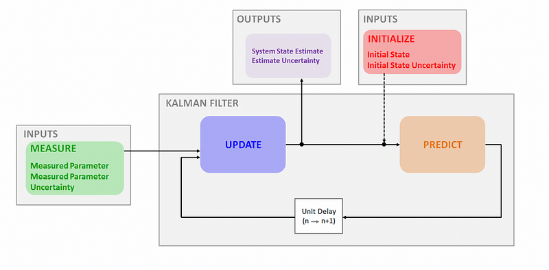
The Kalman Filter requires two primary inputs:
- Initialization - Conducted only once, it includes:
- Initial state
- Initial state uncertainty
Even if the initialization parameters are not accurately defined, the Kalman Filter will converge toward the true value.
- Measurements - Taken during each filtering cycle, these involve:
- Measured system state
- Measurement uncertainty
In addition to the measurements, the filter needs a measurement uncertainty parameter, typically supplied by the equipment manufacturer.
The Kalman Filter operates through a two-step process:
- Prediction Step: It forecasts the next state of the system based on prior measurements.
- Update Step: It assesses the current state of the system based on the latest measurement.
The efficiency of the Kalman Filter lies in its ability to update its predictions using only the information from the previous estimate, thereby requiring minimal computational resources.

Section 1.2: The Operation of Kalman Filter
The Kalman algorithm functions by predicting the system's state for the forthcoming time step. It operates within a "predict-correct" cycle.
Initially, the Kalman Filter is set up with a single initialization step. Once established, it predicts the next state of the system, along with the associated uncertainty. When a new measurement is acquired, the filter adjusts the current state's prediction and its uncertainty.
The prediction process utilizes the existing system state and its uncertainty to forecast the next state, adhering to the system's dynamic model.
Kalman Filter for Beginners, Part 1 - Recursive Filters & MATLAB Examples - YouTube
This tutorial provides an introduction to the Kalman Filter, focusing on recursive filters and demonstrating practical examples using MATLAB.
Conclusion
The Kalman Filter is a powerful yet straightforward algorithm that employs a "predict-correct" methodology for tracking objects. It effectively reduces the computational load required to process noisy input data, yielding more accurate and refined output. By predicting the next system state based on previous measurements and updating it with current measurements, it operates efficiently even with limited resources.
References: