Common Graph Types

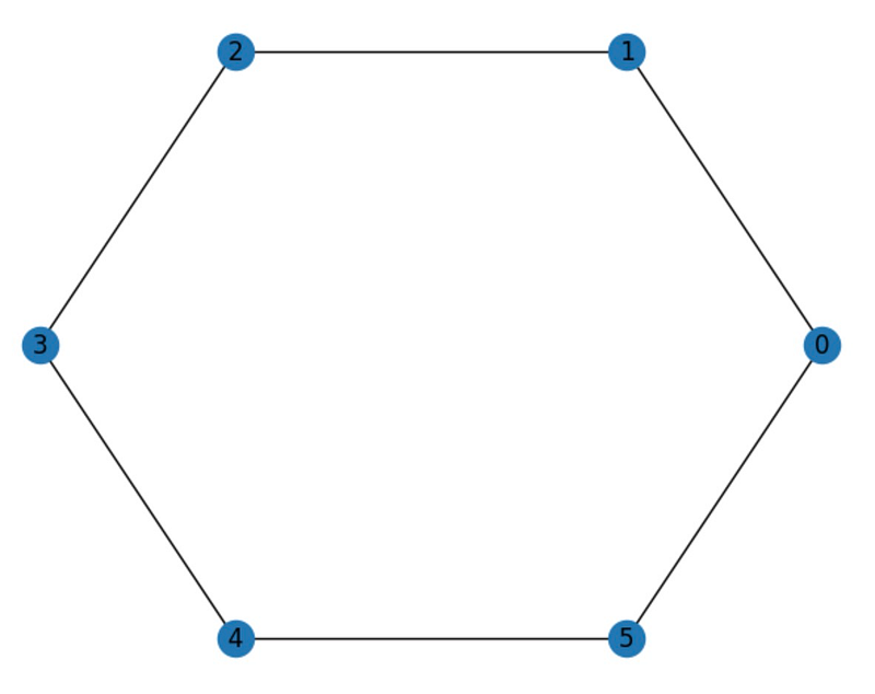
Let’s start by examining a few standard graph types. Circular graphs are drawn in a circle and are often used to represent cyclic or periodic data. In a circular graph, vertices are evenly distributed around the circle, with edges connecting adjacent vertices.

Here’s how to create a circular graph with 6 nodes and 6 edges using networkx's nx.cycle_graph() function, followed by the nx.draw_circular() function to visualize it.

import networkx as nx import matplotlib.pyplot as plt

# Create a circular graph object G = nx.cycle_graph(6)

# Draw the circular graph nx.draw_circular(G, with_labels=True) plt.show()

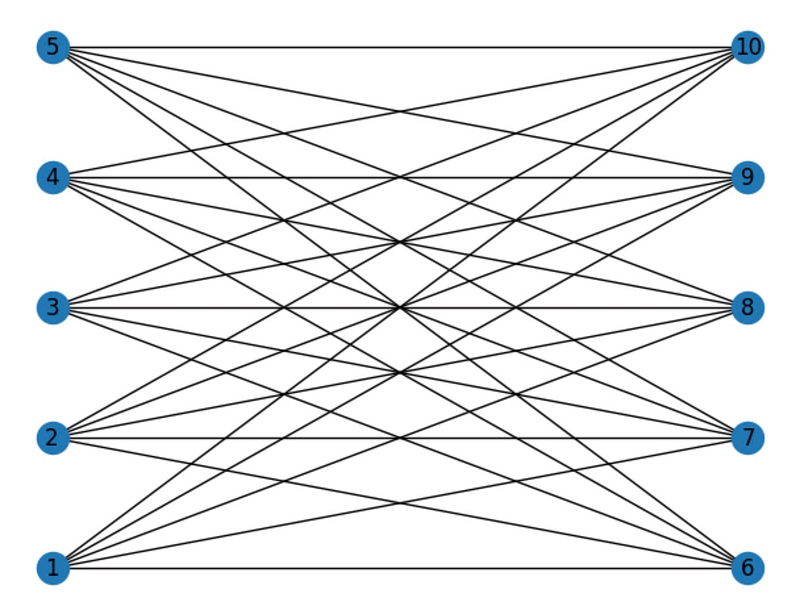
Another prevalent type of graph is the utility graph, often employed to illustrate relationships where one group of objects offers a utility to another group. Each node in a utility graph corresponds to an object from one group, while edges signify connections to objects in the other group.

Here’s an example of a utility graph featuring 5 nodes in each group:

import networkx as nx import matplotlib.pyplot as plt

# Create a utility graph object G = nx.Graph()

# Add nodes to the graph G.add_nodes_from([1, 2, 3, 4, 5], bipartite=0) G.add_nodes_from([6, 7, 8, 9, 10], bipartite=1)

# Connect the nodes for k in range(1, 6):

for j in range(6, 11):

G.add_edge(k, j)

# Draw the utility graph pos = nx.bipartite_layout(G, [1, 2, 3, 4, 5]) nx.draw(G, pos, with_labels=True) plt.show()

In this example, the bipartite option is used to determine which set a node belongs to. A bipartite graph consists of two distinct sets of nodes, where edges only connect nodes from different sets, ensuring no edges exist within the same set.

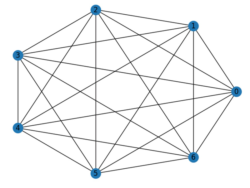
Moving on, let’s consider another widely recognized type of graph—the complete graph. This graph is termed "complete" because every distinct node is connected by an edge. A complete graph with n nodes is denoted as Kn, where n represents the number of nodes. The total count of edges in a complete graph is calculated using the formula n(n-1)/2.

Networkx provides a convenient method to create complete graphs:

import networkx as nx import matplotlib.pyplot as plt

# Create a complete graph object with 7 nodes G = nx.complete_graph(7)

# Draw the complete graph nx.draw_circular(G, with_labels=True) plt.show()

To verify that the number of edges is indeed n(n-1)/2, we can retrieve the edges with:

G.edges

We can also get the nodes using:

G.nodes

This allows us to check our assertion:

n = len(G.nodes) len(G.edges) == n * (n - 1) / 2

This should return True.

Graph Complements

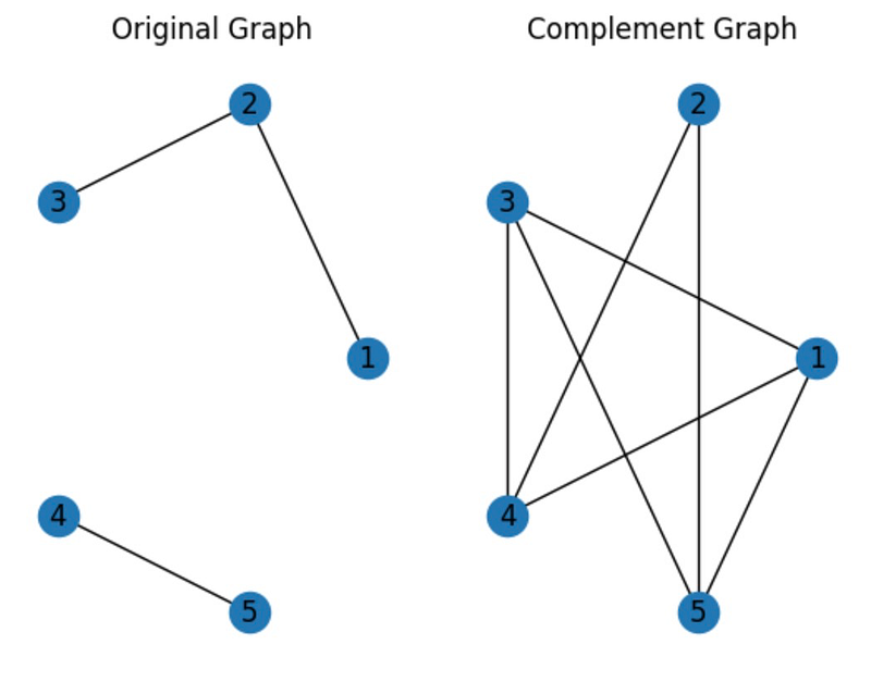
The complement of a graph is another graph that includes all nodes not present in the original graph, while excluding any edges found in the original. If G is the original graph, its complement is denoted as G'.

Here’s an example:

import networkx as nx import matplotlib.pyplot as plt

# Create a graph object with 5 nodes and 3 edges G = nx.Graph() G.add_nodes_from([1, 2, 3, 4, 5]) G.add_edges_from([(1, 2), (2, 3), (4, 5)])

# Create the complement graph G_comp = nx.complement(G)

# Draw both graphs plt.subplot(121) nx.draw_circular(G, with_labels=True) plt.title('Original Graph') plt.subplot(122) nx.draw_circular(G_comp, with_labels=True) plt.title('Complement Graph') plt.show()

Subgraphs

A subgraph is formed by selecting a subset of vertices and edges from a given graph. If G is the original graph, then any graph H derived from G's vertices and edges is a subgraph. This can involve removing certain vertices or edges or choosing a specific subset from G.

To illustrate, here’s an example:

import networkx as nx import matplotlib.pyplot as plt

# Create a graph object with 6 nodes and 7 edges G = nx.Graph() G.add_nodes_from([1, 2, 3, 4, 5, 6]) G.add_edges_from([(1, 2), (2, 3), (3, 4), (4, 5), (5, 6), (6, 1), (2, 4)])

# Create a subgraph by selecting a subset of the edges H = G.edge_subgraph([(1, 2), (2, 3), (3, 4), (4, 5)])

# Draw both graphs plt.subplot(121) nx.draw_circular(G, with_labels=True) plt.title('Original Graph') plt.subplot(122) nx.draw_circular(H, with_labels=True) plt.title('Subgraph') plt.show()

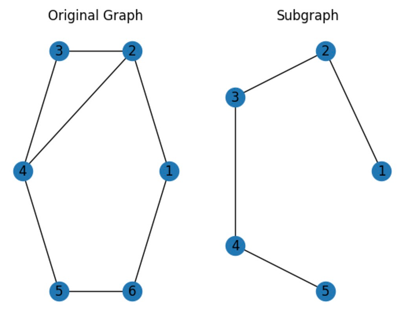
In this case, we've generated a subgraph by using the edge_subgraph() function to include only selected edges from the original graph.

The Degree of a Vertex

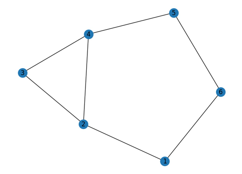
A crucial metric for graph analysis is the degree of a vertex, which indicates how many edges are connected to it. Essentially, it represents the count of other vertices directly linked to that vertex.

To calculate the degree of vertices in networkx, you can use the degree() function:

import networkx as nx import matplotlib.pyplot as plt

# Create a graph object with 6 nodes and 7 edges G = nx.Graph() G.add_nodes_from([1, 2, 3, 4, 5, 6]) G.add_edges_from([(1, 2), (2, 3), (3, 4), (4, 5), (5, 6), (6, 1), (2, 4)])

# Calculate the degree of each vertex degrees = dict(G.degree())

# Print the degree of each vertex for vertex, degree in degrees.items():

print("Vertex", vertex, "has degree", degree)

# Draw the graph nx.draw(G, with_labels=True) plt.show()

Vertex 1 has degree 2 Vertex 2 has degree 3 Vertex 3 has degree 2 Vertex 4 has degree 3 Vertex 5 has degree 2 Vertex 6 has degree 2

The Adjacency Matrix

While graphical representations are beneficial, they may not always be ideal for computational tasks. This is where the adjacency matrix comes in. It is a square matrix that illustrates the connections among graph nodes. The matrix's rows and columns represent the nodes, and the entries indicate the presence of edges between pairs of nodes.

For a graph G with n nodes, the adjacency matrix A is an n x n matrix such that A[i,j] equals 1 if an edge exists from node i to node j, and 0 otherwise. If the graph is undirected, the matrix will be symmetric.

The adjacency matrix is instrumental for graph analysis, enabling quick assessments of node connections, edge counts, and various graph metrics. You can create an adjacency matrix in networkx using the nx.to_numpy_array() function, as shown in the following example:

import networkx as nx import numpy as np

# Create a graph object with 4 nodes and 4 edges G = nx.Graph() G.add_nodes_from([1, 2, 3, 4]) G.add_edges_from([(1, 2), (2, 3), (3, 4), (4, 1)])

# Generate the adjacency matrix adj_mat = nx.to_numpy_array(G)

nx.draw_circular(G, with_labels=True)

# Print the adjacency matrix print(adj_mat)

[[0. 1. 0. 1.]

[1. 0. 1. 0.]

[0. 1. 0. 1.]

[1. 0. 1. 0.]]

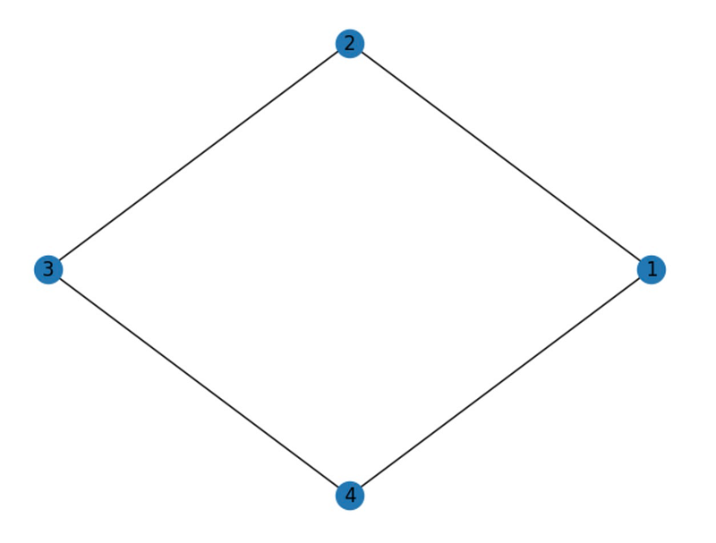
The output reveals a 4 x 4 matrix, where each entry indicates whether an edge exists between two nodes. For instance, the first row and second column entry is 1, signifying an edge between nodes 1 and 2. Since the graph is undirected, the matrix is symmetric.

Cycles in a Graph

A cycle in a graph constitutes a path that starts and ends at the same vertex without revisiting any vertex or edge (excluding the starting and ending vertex). Cycles are pivotal in graph theory for analyzing graph properties and developing algorithms for various graph-related challenges.

In directed graphs, cycles are termed directed cycles or circuits, characterized by paths of directed edges that start and conclude at the same vertex without repeating any node or edge.

Various algorithms, including depth-first search and breadth-first search, can identify cycles. In networkx, you can find cycles using the nx.find_cycle() function:

import networkx as nx

# Create a graph object with 6 nodes and 7 edges G = nx.Graph() G.add_nodes_from([1, 2, 3, 4, 5, 6]) G.add_edges_from([(1, 2), (2, 3), (3, 4), (4, 5), (5, 6), (6, 1), (2, 4)])

# Identify cycles in the graph cycles = nx.cycle_basis(G)

nx.draw_circular(G, with_labels=True)

# Print the cycles print(cycles)

[[2, 4, 5, 6, 1], [2, 3, 4]]

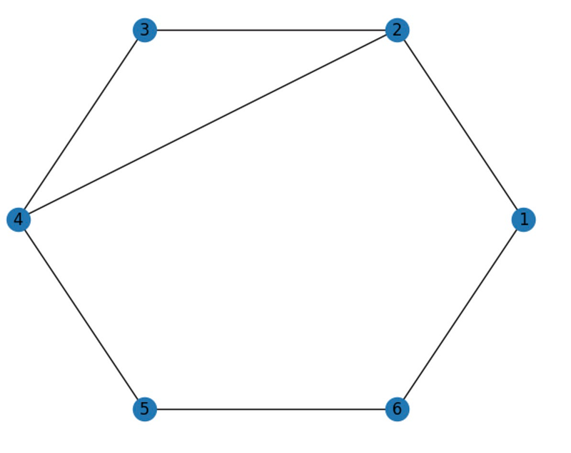
The cycle_basis() function yields a list of cycles present in the graph, with each cycle represented as a list of nodes. The output indicates two cycles in the graph: [2, 4, 5, 6, 1] and [2, 3, 4].

Planarity

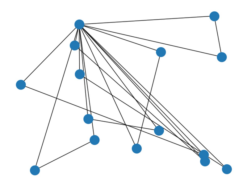
A planar graph can be represented on a two-dimensional plane without edge intersections. Determining if a graph is planar can be complex. For instance, consider the following graph:

import networkx as nx import matplotlib.pyplot as plt

# Create a graph object with 15 nodes G = nx.Graph() G.add_nodes_from(range(1, 16))

# Add the edges G.add_edges_from([(1, 2), (1, 3), (1, 4), (1, 5), (1, 6),

(1, 7), (1, 8), (1, 9), (1, 10), (1, 11),

(1, 12), (1, 13), (1, 14), (1, 15), (2, 3),

(4, 5), (6, 7), (8, 9), (10, 11), (12, 13), (14, 15)])

nx.draw_random(G) plt.show()

In networkx, you can verify the planarity of a graph using the nx.check_planarity() function:

import networkx as nx

K5 = nx.complete_graph(5)

# Check if the graphs are planar G_is_planar, _ = nx.check_planarity(G) K5_is_planar, _ = nx.check_planarity(K5)

print(f"G is planar: {G_is_planar}") print(f"K5 is planar: {K5_is_planar}")

G is planar: True K5 is planar: False

From the results, we see that our graph G is planar, whereas the complete graph with 5 nodes is not.

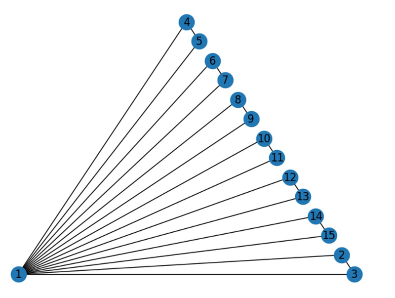
If a graph is planar, networkx can visualize it without edge crossings:

nx.draw_planar(G, with_labels=True)

Conclusion

In summary, graphs are vital tools in mathematics and computer science for modeling relationships among entities. This article has examined several fundamental graph types, including circular graphs, utility graphs, and complete graphs. We also discussed subgraphs, vertex degrees, adjacency matrices, cycles, and planarity. These concepts are integral to graph theory and are applicable in diverse fields, ranging from operations research and social sciences to computer science and network analysis. By leveraging powerful libraries like Python’s networkx, we can efficiently create, visualize, and analyze graphs, providing valuable insights into complex systems.

If you found this article helpful, consider becoming a Medium member for unlimited access to all articles. You can support me as a writer by registering through this link.